Exploring the Many Faces of Power BI Data Models: Star, Snowflake, and Galaxy Schemas
In Power BI, a data model is the foundation of your analysis. It organizes the data, establishes relationships between different tables, and allows for aggregation, filtering, and modeling of your business logic for effective reporting. The way your data model is set up has a significant impact on performance, usability, and the quality of insights you derive from your data.
Below are the types of data models you will typically use in Power BI, their usages, and how to implement them:
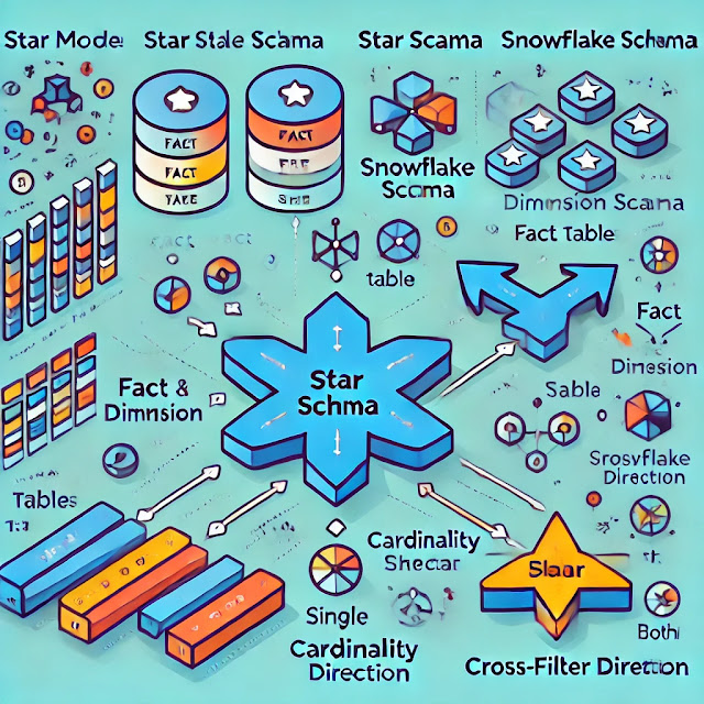
1. Star Schema
- Fact Table: Contains business measurements, usually quantitative data such as sales revenue, quantity sold, or order costs. These tables often have foreign keys that link to dimension tables.
- Dimension Tables: These contain descriptive information that provides context to the measurements in the fact table, such as Customer, Product, or Time.
Example:
- Fact Table: Sales (with fields like Sales_ID, Date_Key, Product_ID, Customer_ID, Sales_Amount)
- Dimension Tables: Time (Date), Product (Product_ID, Name, Category), Customer (Customer_ID, Name, Region)
Implementation in Power BI:
- Import data from the respective sources.
- In the Model View, define relationships (Fact -> Dimensions).
- Set proper cardinality (usually 1:* from Dimension to Fact).
- Configure Date dimension for time intelligence (like Year, Month, Quarter).
Advantages:
- Easy to navigate and understand.
- Efficient querying and calculations.
- Great for BI reports with aggregated data.
2. Snowflake Schema
Structure:
- Fact Table: Like in the star schema, it holds business transaction data.
- Normalized Dimension Tables: Dimensions are further divided into related tables to remove data redundancy. For example, a Product Category dimension might be separated into different tables (ProductCategory, ProductSubcategory, etc.).
Example:
- Fact Table: Sales (Sales_ID, Date_Key, Product_ID, Customer_ID, Sales_Amount)
- Dimension Tables:
- Product (Product_ID, ProductName, ProductSubcategory_ID)
- Product Subcategory (ProductSubcategory_ID, SubcategoryName, ProductCategory_ID)
- Product Category (ProductCategory_ID, CategoryName)
Implementation in Power BI:
- Import data with normalization, creating additional sub-dimension tables.
- Define the relationships in Model View ensuring correct primary-foreign key linkage between normalized tables.
- Perform necessary calculations using DAX (e.g., join columns or use functions like
RELATED()to pull from related tables).
Advantages:
- More normalized data, saving space and avoiding redundancy.
- Easier to maintain when dimensions change.
Disadvantages:
- Can lead to complex relationships.
- Queries may be slower compared to the star schema since more joins are involved.
3. Galaxy Schema (or Fact Constellation Schema)
Structure:
- Contains multiple fact tables and common dimension tables. Dimensions are typically shared across all fact tables (e.g., Product, Customer, Date).
- Example: You might have both Sales and Returns as two fact tables, but both link to common dimension tables like Product, Customer, and Date.
Example:
- Fact Tables: Sales (Sales_ID, Product_ID, Customer_ID, Sales_Amount), Returns (Return_ID, Product_ID, Customer_ID, Return_Amount)
- Shared Dimension Tables: Product (Product_ID, ProductName), Customer (Customer_ID, CustomerName), Date (Date_ID, Year, Month)
Implementation in Power BI:
- Import multiple fact tables with common dimension keys.
- In Model View, create one-to-many relationships from the fact tables to the dimension tables.
- Use aggregation and DAX to create shared measures between the fact tables.
Advantages:
- Useful for businesses with multiple related transactional datasets.
- Allows flexible and consolidated reporting from different perspectives.
Disadvantages:
- More complex structure.
- Can lead to confusion if relationships are not well defined.
4. Flat Model (Denormalized Model)
Structure:
- Data from multiple source tables are combined into one large table. This can include fact data alongside dimensional data.
Sales table containing columns for Sales_ID, ProductName, CustomerName, Sales_Amount, OrderDate, etc., instead of splitting them into separate Product and Customer tables.Implementation in Power BI:
- Import the flat file or denormalized dataset.
- You don’t need to define any relationships since there is only one table.
- Use DAX or Power Query for any necessary transformation or grouping.
Advantages:
- Very simple to implement.
- Fast performance for smaller datasets.
Disadvantages:
- Poor scalability; data duplication increases.
- Difficult to maintain as data grows.
5. One-to-Many with Bridging (Many-to-Many)
Structure:
- Fact Table to Bridge Table (1:*)
- Bridge Table to Dimension Table (many:1)
Implementation in Power BI:
- Create a bridge table.
- Set one-to-many relationships from the fact table to the bridge table and the bridge table to the dimension tables.
- Ensure that you use appropriate DAX functions to aggregate measures across many-to-many links (like
SUMX()).
Advantages:
- Useful for complex many-to-many relationships without data duplication.
- Supports advanced analytics scenarios.
Disadvantages:
- Complex to implement and manage.
- Can increase computational load on large datasets.
Conclusion:
Choosing the right data model for Power BI largely depends on the complexity of the dataset and the business requirements. Here’s a quick summary:
- Star Schema is ideal for simplified, high-performance reporting.
- Snowflake Schema works well when you need normalization and more granular control.
- Galaxy Schema is for businesses with multiple related facts.
- Flat Model is the simplest but not recommended for large, complex datasets.
- One-to-Many with Bridging (Many-to-Many) is useful for complex relationships between entities.
Implementing these models in Power BI involves choosing the right data source, defining relationships in Model View, and creating appropriate measures and calculations using DAX to optimize report performance.


Comments
Post a Comment